🧬 Foundations of Genomic Data Handling in R – Post 9: Biostrings Link to heading

🚀 Why Biostrings? Link to heading

After exploring data structures for genomic ranges and alignments, we now turn to the actual biological sequences themselves. Biostrings is the Bioconductor package that transforms how we work with DNA, RNA, and protein sequences in R, providing memory-efficient storage and high-performance manipulation functions.

Ever tried handling millions of DNA sequences using regular R strings? It quickly becomes unwieldy, slow, and memory-intensive. Biostrings solves these challenges through specialized containers and operations designed specifically for biological sequence data.

🔧 Getting Started with Biostrings Link to heading

Let’s begin with the basics:

# Install if needed
if (!require("BiocManager", quietly = TRUE))
    install.packages("BiocManager")
BiocManager::install("Biostrings")

# Load library
library(Biostrings)

# Create basic DNA sequences
dna1 <- DNAString("ACGTACGTACGT")
dna1

Output:

  12-letter "DNAString" instance
seq: ACGTACGTACGT

Working with multiple sequences is just as straightforward:

# Create a set of DNA sequences (like a FASTA file)
dna_set <- DNAStringSet(c(
  seq1 = "ACGTACGTACGT",
  seq2 = "GTACGTACGTAC",
  seq3 = "AAAAACCCCCGGGGGTTTTTN"
))
dna_set

Output:

DNAStringSet object of length 3:
    width seq                   names               
[1]    12 ACGTACGTACGT          seq1
[2]    12 GTACGTACGTAC          seq2
[3]    21 AAAAACCCCCGGGGGTTTTTN seq3

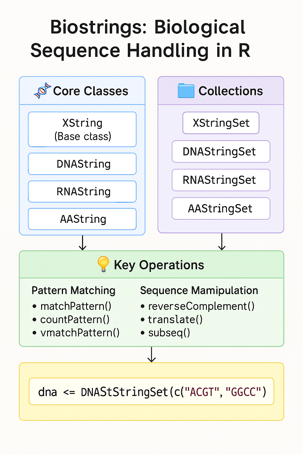
🔍 Key Classes in Biostrings Link to heading

Biostrings provides specialized classes for different biological sequence types:

Core Sequence Classes Link to heading

Collection Classes Link to heading

This class hierarchy enables type-specific operations while maintaining a consistent interface.

⚡ Powerful Operations for Biological Sequences Link to heading

Biostrings provides numerous functions that would be inefficient or difficult with standard string manipulation:

Sequence Information and Statistics Link to heading

# Nucleotide composition
alphabetFrequency(dna_set)

Output:

      A C G T N other
[1,]  3 3 3 3 0     0
[2,]  3 3 3 3 0     0
[3,]  5 5 5 5 1     0

# GC content calculation
letterFrequency(dna_set, letters="GC", as.prob=TRUE)

Output:

         GC
[1,] 0.50000
[2,] 0.50000
[3,] 0.47619

Sequence Manipulation Link to heading

# Reverse complement (fundamental for DNA analysis)
reverseComplement(dna1)

Output:

  12-letter "DNAString" instance
seq: ACGTACGTACGT

# Transcription (DNA to RNA)
transcribe(dna1)

Output:

  12-letter "RNAString" instance
seq: ACGUACGUACGU

# Translation (RNA to protein)
rna <- RNAString("AUGCGAUCGAUCGAUCGAUGAUG")
translate(rna)

Output:

  8-letter "AAString" instance
seq: MRRSIDN*

Pattern Matching Link to heading

# Find all occurrences of a pattern
genome <- DNAString("ACGTACGTAAAACGTACGTTTTACGTACGT")
matchPattern("ACGT", genome)

Output:

Views on a 30-letter DNAString subject
subject: ACGTACGTAAAACGTACGTTTTACGTACGT
views:
     start end width
[1]      1   4     4 [ACGT]
[2]      5   8     4 [ACGT]
[3]     13  16     4 [ACGT]
[4]     17  20     4 [ACGT]
[5]     25  28     4 [ACGT]

# Count occurrences with mismatches allowed
countPattern("ACGT", genome, max.mismatch=1)

Output:

[1] 9

Pairwise Alignment Link to heading

# Align two sequences
seq1 <- DNAString("ACGTACGTACGT")
seq2 <- DNAString("ACGTACGTTTTTACGT")
alignment <- pairwiseAlignment(seq1, seq2)
alignment

Output:

Global PairwiseAlignmentsSingleSubject (1 of 1)
pattern: [1] ACGTACGT-ACGT----- 
subject: [1] ACGTACGTTTTTACGT
score: -6

🔥 Real-world Applications with Code Examples Link to heading

1. Reading and Processing FASTA Files Link to heading

# Read sequences from a FASTA file
sequences <- readDNAStringSet("sequences.fasta")

# Basic sequence stats
sequence_stats <- data.frame(
  Width = width(sequences),
  GC = letterFrequency(sequences, "GC", as.prob=TRUE),
  N_Count = letterFrequency(sequences, "N")
)
head(sequence_stats)

2. Finding Motifs in Genomic Sequences Link to heading

# Define a transcription factor binding site motif
tf_motif <- DNAString("CAAGTG")

# Search for the motif across multiple sequences
motif_positions <- lapply(sequences, function(seq) {
  matches <- matchPattern(tf_motif, seq, max.mismatch=1)
  data.frame(
    Start = start(matches),
    End = end(matches),
    Sequence = as.character(matches)
  )
})

# Count occurrences per sequence
motif_counts <- sapply(motif_positions, nrow)

3. Working with k-mers Link to heading

# Extract all 6-mers from a sequence
generate_kmers <- function(seq, k=6) {
  kmers <- DNAStringSet(
    sapply(1:(length(seq) - k + 1), 
           function(i) subseq(seq, i, i + k - 1))
  )
  return(kmers)
}

# Count k-mer frequencies across sequences
kmers <- generate_kmers(sequences[[1]])
kmer_table <- table(as.character(kmers))
head(sort(kmer_table, decreasing=TRUE))

4. Basic Multiple Sequence Alignment Preparation Link to heading

library(muscle)  # For multiple sequence alignment
library(DECIPHER)  # Another option for MSA

# Align sequences
aligned <- DNAStringSet(muscle::muscle(sequences))

# Extract conserved regions
consensus <- consensusMatrix(aligned, as.prob=TRUE)
conservation <- rowSums(apply(consensus, 1, function(x) sort(x, decreasing=TRUE)[1]))
conserved_positions <- which(conservation > 0.9)

💯 Performance Benefits Link to heading

Biostrings offers substantial performance advantages over standard R:

Memory Efficiency Link to heading

DNA sequences require only 2 bits per base (instead of 8 bits per character in standard strings):

# Compare memory usage
standard_string <- paste(rep("ACGT", 250000), collapse="")
dna_string <- DNAString(standard_string)

object.size(standard_string)  # ~1MB
object.size(dna_string)       # ~250KB (75% reduction)

Speed Improvements Link to heading

Operations are dramatically faster, especially for pattern matching:

# Create a larger sequence for testing
large_seq <- paste(rep("ACGTACGTACGT", 100000), collapse="")
large_dna <- DNAString(large_seq)

# Standard R approach (much slower)
system.time(gregexpr("ACGT", large_seq))

# Biostrings approach (much faster)
system.time(matchPattern("ACGT", large_dna))

Key Performance Advantages Link to heading

• Compact storage: 2-bit encoding for DNA/RNA sequences
• Vectorized operations: Optimized C code for common sequence manipulations
• Specialized algorithms: Implementations tailored for biological sequences
• Efficient views: No-copy access to sequence subsets
• Type safety: Prevents invalid operations on sequences

🧬 Why Biostrings Matters Link to heading

Biostrings transforms tedious and inefficient sequence handling into elegant, performant operations. It provides:

• Biological relevance: Operations designed for DNA, RNA, and protein analysis
• Scale handling: Efficiently works with sequences from PCR products to entire genomes
• Integration: Connects seamlessly with other Bioconductor packages like GenomicRanges
• Comprehensiveness: Covers everything from basic manipulation to complex pattern matching
• Performance: Optimized for the unique characteristics of biological sequence data

Whether you’re analyzing a few sequences or building a genome-wide analysis pipeline, Biostrings provides the solid foundation needed for efficient biological sequence manipulation in R.

🧪 What’s Next? Link to heading

Coming up: BSgenome — accessing complete reference genomes in R, built on the foundation of Biostrings for seamless navigation and extraction of genomic sequences! 🎯

💬 Share Your Thoughts! Link to heading

How are you using Biostrings in your genomic workflows? Any tips for optimizing sequence analysis? Drop a comment below! 👇

#Bioinformatics #RStats #Biostrings #SequenceAnalysis #Bioconductor #DNA #RNA #Protein #GenomicAnalysis #ComputationalBiology #Genomics #BiologicalSequences