🧬 Foundations of Genomic Data Handling in R – Post 10: plyranges Link to heading
🚀 Why plyranges? Link to heading
After exploring the core Bioconductor infrastructure for genomic ranges, alignments, and sequences, it’s time to discover how modern R programming paradigms can transform our workflows. plyranges bridges the gap between Bioconductor’s powerful genomic tools and the intuitive tidyverse syntax that R users love.
Remember when genomic range operations required pages of complex, hard-to-read code with nested function calls? plyranges changed the game by bringing tidyverse elegance to genomic data analysis. It transforms the way we interact with GRanges objects, making genomic analyses more readable, maintainable, and fun!
🔧 Getting Started with plyranges Link to heading
First, install and load the required packages:
# Install if needed
if (!require("BiocManager", quietly = TRUE))
    install.packages("BiocManager")
BiocManager::install("plyranges")

# Load libraries
library(plyranges)
library(GenomicRanges)
Let’s create a simple GRanges object and apply some basic plyranges operations:
# Create a basic GRanges object
gr <- GRanges(
  seqnames = "chr1",
  ranges = IRanges(start = 1:5, width = 10),
  strand = c("+", "+", "*", "-", "-"),
  score = 1:5
)

# Apply plyranges operations with pipes
gr_filtered <- gr %>%
  filter(start > 2) %>%
  mutate(score_doubled = score * 2) %>%
  select(score, score_doubled)

gr_filtered
Output:
GRanges object with 3 ranges and 2 metadata columns:
      seqnames    ranges strand |     score score_doubled
         <Rle> <IRanges>  <Rle> | <integer>     <numeric>
  [1]     chr1     3-12      * |         3             6
  [2]     chr1     4-13      - |         4             8
  [3]     chr1     5-14      - |         5            10
  -------
  seqinfo: 1 sequence from an unspecified genome; no seqlengths
The transformation is remarkable – what would have been multiple nested function calls becomes a linear, readable pipeline.
🔍 Key Features of plyranges Link to heading
plyranges reimagines genomic range manipulation through familiar tidyverse-style verbs:
1. Filtering and Subsetting Ranges Link to heading
# Filter based on range properties
gr %>% filter(width > 5, strand == "+")

# Filter based on metadata
gr %>% filter(score > 3)

# Slice to select specific ranges
gr %>% slice(2:4)
2. Adding and Transforming Metadata Link to heading
# Add new metadata columns
gr %>%
  mutate(
    category = ifelse(score > 3, "high", "low"),
    gc_content = runif(length(gr), 0.3, 0.6)
  )

# Modify existing columns
gr %>% mutate(score = score / max(score))
3. Genomic Range Operations Link to heading
# Shift ranges by 1000bp
gr %>% mutate(start = start + 1000, end = end + 1000)

# More elegant with specialized functions
gr %>% shift_right(1000)

# Resize ranges
gr %>% mutate(width = 100)  # or
gr %>% resize(width = 100)

# Create flanking regions
gr %>% flank_left(width = 50)  # 50bp upstream
4. Joining Genomic Ranges Link to heading
One of the most powerful features is the intuitive syntax for overlap operations:
# Create another set of ranges
gr2 <- GRanges(
  seqnames = "chr1",
  ranges = IRanges(start = c(3, 8, 15), width = 5),
  strand = c("+", "*", "-"),
  type = c("enhancer", "promoter", "gene")
)

# Find overlaps between ranges (like SQL INNER JOIN)
gr %>% join_overlap_inner(gr2)

# Overlap with additional constraints
gr %>% join_overlap_inner(gr2, maxgap = 2)  # Allow 2bp gap

# Find ranges in gr that overlap gr2 (like SQL LEFT JOIN)
gr %>% join_overlap_left(gr2)

# Find ranges in gr that don't overlap gr2
gr %>% join_overlap_inner_not(gr2)
5. Grouping and Summarizing Link to heading
plyranges extends the group-by operations to genomic contexts:
# Group by strand and summarize
gr %>%
  group_by(strand) %>%
  summarize(
    count = n(),
    mean_score = mean(score),
    total_width = sum(width)
  )
Output:
GRanges object with 3 ranges and 3 metadata columns:
      seqnames    ranges strand |     count mean_score total_width
         <Rle> <IRanges>  <Rle> | <integer>  <numeric>   <integer>
  [1]     chr1        NA      + |         2        1.5          20
  [2]     chr1        NA      * |         1        3.0          10
  [3]     chr1        NA      - |         2        4.5          20
  -------
  seqinfo: 1 sequence from an unspecified genome; no seqlengths
💯 Real-World Applications with Code Examples Link to heading
Let’s explore some practical genomic analysis workflows using plyranges:
1. Finding Promoters Overlapping ChIP-seq Peaks Link to heading
library(TxDb.Hsapiens.UCSC.hg19.knownGene)
library(plyranges)

# Get gene models
genes <- genes(TxDb.Hsapiens.UCSC.hg19.knownGene)

# Define promoters (2kb upstream)
promoters <- genes %>% promoters(upstream = 2000, downstream = 200)

# Read ChIP-seq peaks from BED file
peaks <- read_bed("chipseq_peaks.bed")

# Find promoters with overlapping peaks and count peaks per gene
promoter_peaks <- promoters %>%
  join_overlap_inner(peaks) %>%
  group_by(gene_id) %>%
  summarize(peak_count = n()) %>%
  arrange(desc(peak_count))

# Display top genes by peak count
head(promoter_peaks)
2. Filtering and Classifying Genomic Features Link to heading
# Read genomic features
features <- read_gff("annotations.gff")

# Complex filtering and annotation
filtered_features <- features %>%
  filter(type == "exon", width > 100) %>%
  mutate(
    gc_content = calculate_gc(sequence),  # Hypothetical function
    size_class = case_when(
      width < 200 ~ "small",
      width < 500 ~ "medium",
      TRUE ~ "large"
    )
  ) %>%
  filter(gc_content > 0.4) %>%
  select(gene_id, transcript_id, size_class, gc_content)

# Summarize by size class
filtered_features %>%
  group_by(size_class) %>%
  summarize(
    count = n(),
    mean_gc = mean(gc_content),
    mean_width = mean(width)
  )
3. Finding Distance to Nearest Feature Link to heading
# Find closest genes to each peak
nearest_genes <- peaks %>%
  join_nearest(genes) %>%
  mutate(
    distance = distance_to_nearest(genes),
    regulation = case_when(
      strand == "+" & start(genes) > end ~ "upstream",
      strand == "-" & start(genes) < start ~ "upstream",
      TRUE ~ "downstream"
    )
  ) %>%
  select(peak_id, gene_id, distance, regulation)

# Tabulate regulatory relationships
table(nearest_genes$regulation)
4. Finding Differentially Accessible Regions Link to heading
# Combine ATAC-seq peaks from multiple conditions
condition1 <- read_bed("condition1_peaks.bed") %>% mutate(condition = "treatment")
condition2 <- read_bed("condition2_peaks.bed") %>% mutate(condition = "control")

# Combine peaks
all_peaks <- bind_ranges(condition1, condition2)

# Find consensus peaks
consensus <- all_peaks %>%
  reduce_ranges() %>%
  mutate(peak_id = paste0("peak_", 1:length(.)))

# Count peaks per condition in each consensus region
peak_matrix <- consensus %>%
  join_overlap_left(all_peaks) %>%
  group_by(peak_id, condition) %>%
  summarize(count = n()) %>%
  pivot_wider(names_from = condition, values_from = count, values_fill = 0)

# Identify differential peaks
differential_peaks <- peak_matrix %>%
  filter(treatment > 0 | control > 0) %>%
  mutate(
    log2FC = log2((treatment + 1) / (control + 1)),
    status = case_when(
      log2FC > 1 ~ "treatment_specific",
      log2FC < -1 ~ "control_specific",
      TRUE ~ "shared"
    )
  )
🧠 Why plyranges Matters Link to heading
plyranges represents more than just a syntactic convenience—it’s a paradigm shift in how we approach genomic data analysis:
1. Code Readability and Maintainability Link to heading
Compare the traditional approach:
# Traditional nested approach
subset(
  mcols(
    resize(
      shift(
        subset(gr, strand == "+" & score > 3),
        1000
      ),
      width = 500,
      fix = "center"
    )
  ),
  select = c("score", "gc_content")
)
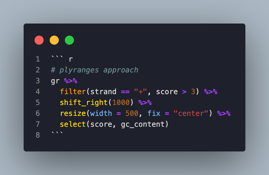
With the plyranges approach:
# plyranges approach
gr %>%
  filter(strand == "+", score > 3) %>%
  shift_right(1000) %>%
  resize(width = 500, fix = "center") %>%
  select(score, gc_content)
The difference is striking—the plyranges version reads like a story, making it easier to understand, debug, and maintain.
2. Integration with Both Ecosystems Link to heading
plyranges creates a seamless bridge between two powerful R ecosystems: - Leverages the rich genomic functionality of Bioconductor - Adopts the intuitive grammar of the tidyverse
This integration allows analysts familiar with either ecosystem to quickly become productive.
3. Lowering the Learning Curve Link to heading
By using consistent, meaningful verbs across operations, plyranges reduces the cognitive load required to work with genomic data: - Same verbs apply to different genomic operations - Intuitive function names reflect their purpose - Consistent argument patterns across functions
4. Improved Reproducibility Link to heading
Clear, readable code enhances reproducibility by: - Making the analysis intention obvious - Reducing errors from complex nested syntax - Facilitating code review and collaboration - Enabling clearer documentation in publications
🎯 plyranges in the Genomic Ecosystem Link to heading
plyranges integrates seamlessly with other Bioconductor tools:
- GenomicRanges: Enhances the core functionality without replacing it
- rtracklayer: Import/export functions like
read_bed()andread_gff() - BSgenome: Simplified extraction of sequences from reference genomes
- SummarizedExperiment: Streamlined manipulation of feature annotations
- GenomicFeatures: Fluent interfaces for gene model manipulation
plyranges demonstrates the power of bringing modern programming paradigms to specialized domains — a true game-changer that has made genomic data analysis more intuitive and productive.
🧪 What’s Next? Link to heading
Coming up: SummarizedExperiment — bringing it all together for a unified container integrating assay data with genomic coordinates and sample information! 🎯
💬 Share Your Thoughts! Link to heading
How has plyranges transformed your genomic data analysis workflows? Any favorite tricks for simplifying complex operations? Drop a comment below! 👇
#Bioinformatics #RStats #plyranges #tidyverse #GenomicRanges #Bioconductor #DataManipulation #Genomics #ComputationalBiology #DataScience