🧬 Foundations of Genomic Data Handling in R – Post 11: rtracklayer Link to heading
🚀 Why rtracklayer? Link to heading
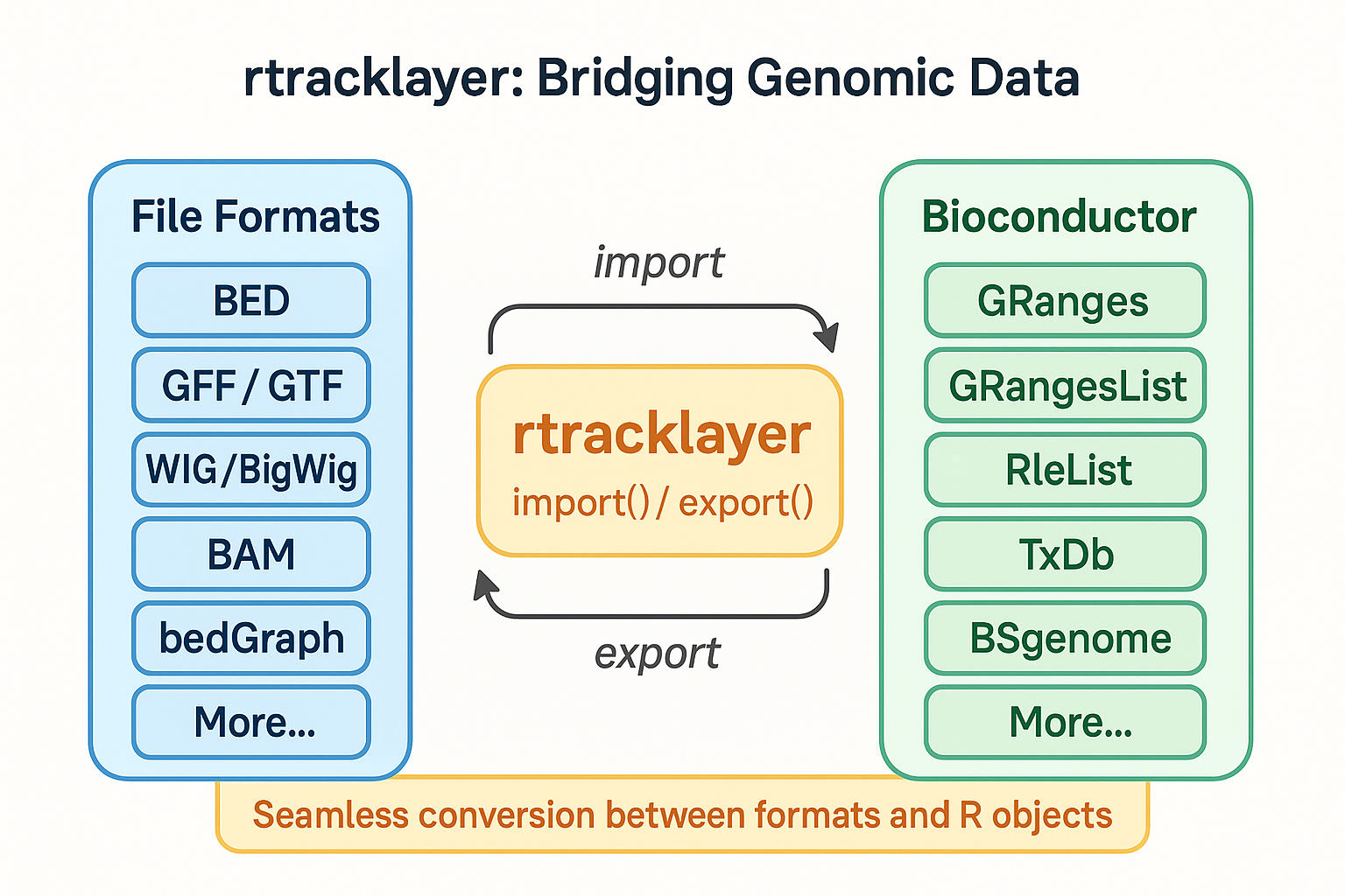
After exploring the core Bioconductor data structures and manipulation tools, we need to address a critical question: How do we get genomic data into R from the diverse ecosystem of file formats? This is where rtracklayer shines. It serves as the Swiss Army knife of genomic data I/O, providing a unified interface for importing, exporting, and converting between genomic file formats.
Ever struggled with writing custom parsers for BED files, then having to write different code for GTF, WIG, or bigWig files? rtracklayer eliminates this hassle with a consistent API that seamlessly connects the outside world of genomic data to the structured environment of Bioconductor.
🔧 Getting Started with rtracklayer Link to heading
Let’s begin with basic import/export operations:
# Install if needed
if (!require("BiocManager", quietly = TRUE))
    install.packages("BiocManager")
BiocManager::install("rtracklayer")

# Load library
library(rtracklayer)
library(GenomicRanges)

# Import different file formats with a unified interface
peaks <- import("chipseq_peaks.bed")
genes <- import("annotations.gtf")
coverage <- import("signal.bigWig")

# Export is just as straightforward
export(peaks, "peaks.gff3")
The beauty of rtracklayer is that it automatically converts files to appropriate Bioconductor objects—typically GRanges or GRangesList—regardless of the input format. This creates a consistent foundation for downstream analysis.
🔍 Supported File Formats Link to heading
rtracklayer handles a wide range of genomic file formats:
| Format | Type | Import | Export | Common Use |
|---|---|---|---|---|
| BED | Range | ✓ | ✓ | Peak calls, generic annotations |
| GFF/GTF | Range | ✓ | ✓ | Gene annotations, features |
| WIG | Score | ✓ | ✓ | Continuous signal data |
| bigWig | Score | ✓ | ✓ | Compressed signal tracks |
| bedGraph | Score | ✓ | ✓ | Sparse signal representation |
| 2bit | Sequence | ✓ | ✓ | Compressed DNA sequence |
| BAM (header) | Range | ✓ | ✗ | Alignment metadata |
| VCF | Range | ✓ | ✓ | Variant calls |
| BroadPeak | Range | ✓ | ✓ | ENCODE peak format |
| narrowPeak | Range | ✓ | ✓ | ENCODE peak format |
Each format is converted to an appropriate Bioconductor object: - Range formats (BED, GFF) → GRanges - Hierarchical formats (GTF) → GRangesList - Signal formats (WIG, bigWig) → GRanges with score metadata - Sequence formats → DNAStringSet
⚡ Key Features and Practical Applications Link to heading
1. Selective Imports with Range Filtering Link to heading
One of rtracklayer’s most powerful features is the ability to selectively import regions from huge files:
# Define a region of interest
region_of_interest <- GRanges("chr1", IRanges(1000000, 2000000))

# Import only genes in this region (memory efficient!)
genes_of_interest <- import("genome.gtf", which = region_of_interest)

# Similarly for signal data
signal_subset <- import("chip.bigWig", which = region_of_interest)
This selective import is crucial for working with genome-scale files that would otherwise exhaust memory.
2. Format Conversion Link to heading
Converting between formats becomes trivial:
# Import peaks from BED format
peaks <- import("peaks.bed")

# Export as different formats
export(peaks, "peaks.gff3")
export(peaks, "peaks.bedGraph", format = "bedGraph")
export(peaks, "peaks.bigBed", format = "bigBed")
The format parameter can override the default format inferred from the file extension.
3. Working with Genome Browsers Link to heading
rtracklayer even provides functions to interact with genome browsers:
# Create a track for UCSC browser
track <- DataTrack(peaks, name = "My ChIP-seq Peaks",
                  description = "HeLa H3K4me3 peaks")

# Create a browser URL
ucscTrackMeta(track)
4. Integration with GenomicFeatures Link to heading
rtracklayer works seamlessly with other Bioconductor packages:
library(GenomicFeatures)

# Import gene annotations
genes <- import("gencode.v38.annotation.gtf")

# Convert to TxDb for advanced gene model operations
txdb <- makeTxDbFromGRanges(genes)

# Extract exons by gene
exons_by_gene <- exonsBy(txdb, by = "gene")

# Export selected features
export(transcripts(txdb), "transcripts.bed")
5. Signal Extraction from BigWig Files Link to heading
rtracklayer excels at extracting and summarizing signal data:
# Import gene annotations and get promoters
genes <- import("annotations.gtf")
promoters <- promoters(genes, upstream = 2000, downstream = 200)

# Get signal over promoters
promoter_signal <- import("chip.bigWig", which = promoters)

# Calculate mean signal per promoter
library(GenomicRanges)
hits <- findOverlaps(promoters, promoter_signal)
promoter_means <- tapply(
  mcols(promoter_signal)$score[subjectHits(hits)],
  queryHits(hits),
  mean
)

# Add mean signal to promoters
mcols(promoters)$mean_signal <- NA
mcols(promoters)$mean_signal[as.integer(names(promoter_means))] <- promoter_means
💯 Efficiency Considerations Link to heading
Working with large genomic files can be challenging. Here are some rtracklayer best practices:
1. Use Range Restrictions Link to heading
Always use the which parameter when targeting specific regions:
# Bad: Loads entire genome file
whole_genome <- import("hg38.bigWig")

# Good: Only loads chromosome 1
chr1_only <- import("hg38.bigWig", which = GRanges("chr1", IRanges(1, 248956422)))
2. Leverage BigWig and BigBed for Large Datasets Link to heading
# Convert large WIG file to compressed bigWig
wig_data <- import("large_dataset.wig")
export(wig_data, "large_dataset.bigWig")

# Future imports will be faster and more memory-efficient
compressed_data <- import("large_dataset.bigWig")
3. Chunk Processing for Enormous Files Link to heading
For truly massive files, process in chunks:
# Process genome by chromosome
chromosomes <- paste0("chr", c(1:22, "X", "Y"))
result_list <- list()

for (chr in chromosomes) {
  chr_range <- GRanges(chr, IRanges(1, 5e8))  # Large enough for any chromosome
  chunk <- import("enormous.bigWig", which = chr_range)
  result_list[[chr]] <- processChunk(chunk)  # Your processing function
}

# Combine results
final_result <- do.call(c, result_list)
🧠 Why rtracklayer Matters Link to heading
rtracklayer serves as the critical bridge between the diverse world of genomic file formats and the structured analytical environment of Bioconductor. Its importance stems from several key aspects:
1. Format Unification Link to heading
Genomics has evolved with many specialized file formats for different data types. rtracklayer unifies these behind a consistent interface, eliminating the need for format-specific code.
2. Memory Management Link to heading
Through selective imports and support for compressed formats like bigWig, rtracklayer enables the analysis of datasets that would otherwise be impossibly large for R.
3. Integration with Bioconductor Ecosystem Link to heading
By converting various formats to GRanges objects, rtracklayer creates immediate compatibility with the entire universe of Bioconductor tools.
4. Reproducibility Link to heading
Explicit import and export operations in your scripts make workflow reproducibility straightforward—the exact same data is loaded in exactly the same way.
5. Rapid Prototyping Link to heading
The ability to quickly import, manipulate, and export different formats accelerates the development of genomic analysis pipelines.
🎯 Real-World Example: Complete ChIP-seq Analysis Workflow Link to heading
Here’s how rtracklayer fits into a complete ChIP-seq analysis workflow:
# Import peak calls
peaks <- import("chipseq_peaks.bed")

# Import gene annotations
genes <- import("gencode.gtf")

# Get promoters
promoters <- promoters(genes[genes$type == "gene"], upstream=2000, downstream=200)

# Find peaks overlapping promoters
library(GenomicRanges)
peak_promoter_overlaps <- findOverlaps(peaks, promoters)
promoter_peaks <- peaks[queryHits(peak_promoter_overlaps)]
genes_with_peaks <- genes[genes$type == "gene"][subjectHits(peak_promoter_overlaps)]

# Import signal track
signal <- import("chipseq_signal.bigWig")

# Summarize signal over peaks
peak_signal <- signal[findOverlaps(signal, promoter_peaks, select="first")]

# Export results in formats suitable for other tools
export(promoter_peaks, "promoter_peaks.bed")
export(genes_with_peaks, "genes_with_peaks.gtf")

# Create genome browser visualization files
export(coverage(peak_signal), "peak_coverage.bigWig")
This workflow seamlessly combines imports, genomic range operations, and exports through rtracklayer’s unified interface.
🧪 What’s Next? Link to heading
Coming up: SummarizedExperiment — the container that brings everything together, integrating assay data with genomic coordinates and sample information into a comprehensive package for genomic data analysis! 🎯
💬 Share Your Thoughts! Link to heading
How has rtracklayer simplified your genomic data workflows? Any tips for handling particularly challenging file formats? Drop a comment below! 👇
#Bioinformatics #RStats #rtracklayer #Bioconductor #GenomicRanges #DataImport #FileFormats #BAM #BED #GTF #WIG #NGS #ComputationalBiology