🧬 Foundations of Genomic Data Handling in R – Post 13: SummarizedExperiment Link to heading
🚀 The Masterpiece Container Link to heading
After our journey through the foundational components of Bioconductor—from GRanges and DataFrame to plyranges and rtracklayer—we arrive at the masterpiece that brings it all together: SummarizedExperiment. This isn’t just another data structure; it’s the culmination of thoughtful design that unifies genomic coordinates, experimental measurements, and metadata into a single, powerful object.
SummarizedExperiment represents the standard container for RNA-seq, ChIP-seq, ATAC-seq, and virtually every experimental genomics workflow in Bioconductor. It elegantly solves the fundamental challenge of keeping experimental data, genomic coordinates, and sample information synchronized—preventing the nightmare of mismatched annotations that plague many genomic analyses.
Think of SummarizedExperiment as the Swiss Army knife of experimental genomics: it contains everything you need in one unified, well-organized package.
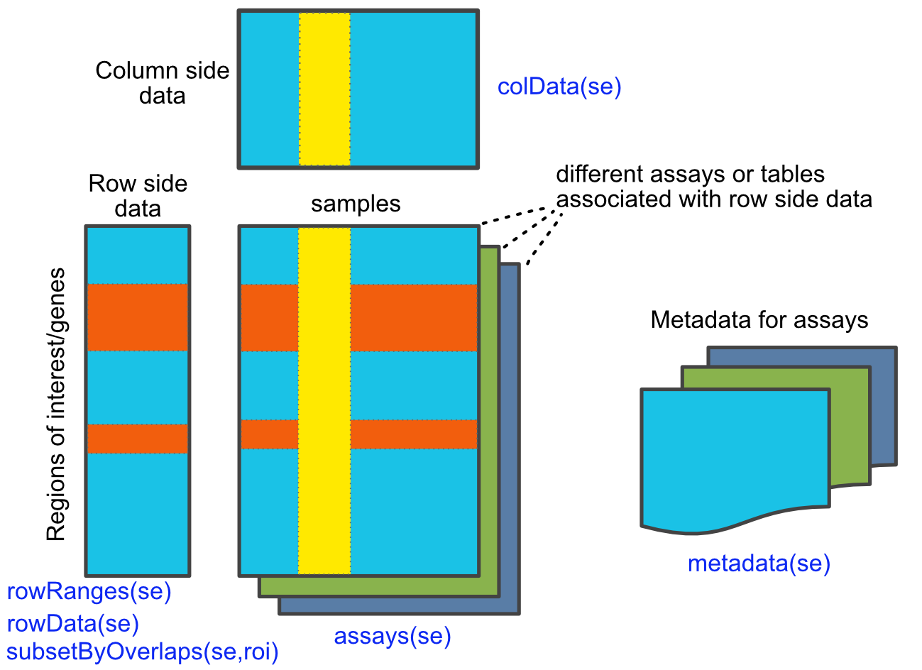
🔧 The Elegant Three-Part Architecture Link to heading
SummarizedExperiment is built around three core components that should feel familiar from our series:
# Install if needed
if (!require("BiocManager", quietly = TRUE))
    install.packages("BiocManager")
BiocManager::install("SummarizedExperiment")

# Load libraries
library(SummarizedExperiment)
library(GenomicRanges)

# Create a basic SummarizedExperiment
se <- SummarizedExperiment(
  assays = list(counts = count_matrix),
  rowRanges = gene_granges,
  colData = sample_metadata
)
Let’s create a concrete example to illustrate each component:
1. Assays: The Experimental Measurements Link to heading
# Create a count matrix (genes x samples)
set.seed(123)
count_matrix <- matrix(
  rpois(60, lambda = 10),
  nrow = 6, ncol = 10,
  dimnames = list(
    paste0("gene", 1:6),
    paste0("sample", 1:10)
  )
)

# Multiple assays are common (raw counts, normalized, etc.)
normalized_matrix <- log2(count_matrix + 1)
2. rowRanges: Genomic Coordinates (Our GRanges Foundation!) Link to heading
# Create genomic ranges for our features
gene_ranges <- GRanges(
  seqnames = rep(c("chr1", "chr2"), each = 3),
  ranges = IRanges(
    start = c(1000, 5000, 10000, 2000, 8000, 15000),
    width = c(2000, 1500, 3000, 1800, 2200, 2500)
  ),
  strand = rep(c("+", "-"), each = 3),
  gene_id = paste0("gene", 1:6),
  symbol = paste0("SYMBOL", 1:6),
  biotype = rep(c("protein_coding", "lncRNA"), 3)
)
3. colData: Sample Information (Our DataFrame Structures!) Link to heading
# Create sample metadata
sample_info <- DataFrame(
  sample_id = paste0("sample", 1:10),
  condition = rep(c("control", "treatment"), each = 5),
  batch = rep(1:2, 5),
  sex = sample(c("Male", "Female"), 10, replace = TRUE),
  age = sample(25:65, 10, replace = TRUE)
)
Now we can create our complete SummarizedExperiment:
# Combine everything
se <- SummarizedExperiment(
  assays = list(
    counts = count_matrix,
    logcounts = normalized_matrix
  ),
  rowRanges = gene_ranges,
  colData = sample_info
)

# Examine the object
se
Output:
class: SummarizedExperiment
dim: 6 10
assays(2): counts logcounts
rownames(6): gene1 gene2 gene3 gene4 gene5 gene6
rowData names(3): gene_id symbol biotype
colnames(10): sample1 sample2 ... sample9 sample10
colData names(5): sample_id condition batch sex age
🔍 Accessing and Manipulating Data Link to heading
SummarizedExperiment provides intuitive accessors that connect to everything we’ve learned:
Accessing Components Link to heading
# Access assay data
assay(se, "counts")           # First assay
assay(se, "logcounts")        # Named assay
assays(se)                    # All assays

# Access genomic coordinates (our GRanges!)
rowRanges(se)

# Access sample information (our DataFrame!)
colData(se)

# Access feature metadata
rowData(se)  # Same as mcols(rowRanges(se))
Elegant Subsetting Link to heading
The real power comes from synchronized subsetting:
# Subset by genomic location
chr1_genes <- se[seqnames(se) == "chr1", ]

# Subset by feature properties
protein_coding <- se[rowData(se)$biotype == "protein_coding", ]

# Subset by sample characteristics
treated_samples <- se[, colData(se)$condition == "treatment"]

# Complex combined subsetting
filtered <- se[
  rowData(se)$biotype == "protein_coding" & width(se) > 2000,
  colData(se)$condition == "treatment" & colData(se)$age > 40
]
Notice how the rows and columns are automatically synchronized—no risk of mismatched annotations!
⚡ Integration with Our Foundational Series Link to heading
Let’s see how SummarizedExperiment integrates with all the packages we’ve explored:
1. plyranges Integration Link to heading
library(plyranges)

# Use plyranges syntax on SummarizedExperiment
se %>%
  filter(seqnames == "chr1") %>%
  mutate(mean_expression = rowMeans(assay(., "counts"))) %>%
  select(gene_id, symbol, mean_expression)
2. rtracklayer Integration Link to heading
library(rtracklayer)

# Export feature ranges
export(rowRanges(se), "features.bed")

# Import additional annotations and add to the object
new_annotations <- import("additional_features.gtf")
rowRanges(se) <- rowRanges(se)[findOverlaps(rowRanges(se), new_annotations, select="first")]
3. GenomicAlignments Connection Link to heading
# SummarizedExperiment often created from alignment summaries
library(GenomicAlignments)

# Count reads in features (typical RNA-seq workflow)
bam_files <- BamFileList(c("sample1.bam", "sample2.bam"))
gene_counts <- summarizeOverlaps(
  features = gene_ranges,
  reads = bam_files,
  mode = "Union"
)
# gene_counts is already a SummarizedExperiment!
💯 Real-World Applications Link to heading
1. RNA-seq Analysis Workflow Link to heading
# Complete RNA-seq analysis setup
library(DESeq2)

# SummarizedExperiment flows directly into DESeq2
dds <- DESeqDataSet(se, design = ~ condition + batch)

# Filter low-count genes using genomic information
keep <- rowSums(assay(dds) >= 10) >= 3 & width(dds) > 500
dds_filtered <- dds[keep, ]

# Run differential expression
dds_analyzed <- DESeq(dds_filtered)

# Results include genomic coordinates automatically
results_df <- results(dds_analyzed) %>%
  as.data.frame() %>%
  cbind(as.data.frame(rowRanges(dds_analyzed)))
2. Multi-Assay Integration Link to heading
# Adding multiple data types to the same experiment
se_multi <- se

# Add protein abundance data
assay(se_multi, "protein") <- matrix(
  runif(60, 0, 100),
  nrow = 6, ncol = 10,
  dimnames = dimnames(count_matrix)
)

# Add ChIP-seq signal
assay(se_multi, "h3k4me3") <- matrix(
  runif(60, 0, 50),
  nrow = 6, ncol = 10,
  dimnames = dimnames(count_matrix)
)

# Now we can analyze relationships between data types
cor(assay(se_multi, "counts")[1, ], assay(se_multi, "protein")[1, ])
3. Genomic Context Analysis Link to heading
# Use genomic coordinates for context analysis
library(TxDb.Hsapiens.UCSC.hg19.knownGene)

# Get promoter regions
promoters <- promoters(TxDb.Hsapiens.UCSC.hg19.knownGene)

# Find genes with promoter overlap
promoter_overlaps <- findOverlaps(rowRanges(se), promoters)

# Add promoter information
rowData(se)$has_promoter <- seq_len(nrow(se)) %in% queryHits(promoter_overlaps)

# Analyze expression by genomic context
boxplot(rowMeans(assay(se, "counts")) ~ rowData(se)$has_promoter,
        ylab = "Mean Expression", xlab = "Has Promoter Overlap")
🎯 The Complete Integration Story Link to heading
Let’s trace the complete data flow that brings together our entire series:
1. Data Generation and Quality Control Link to heading
# Start with raw sequencing data (ShortRead)
library(ShortRead)
raw_reads <- readFastq("sample.fastq")
clean_reads <- raw_reads[quality_filter(raw_reads)]
2. Sequence Processing Link to heading
# Extract and manipulate sequences (Biostrings)
library(Biostrings)
sequences <- sread(clean_reads)
gc_content <- letterFrequency(sequences, "GC", as.prob = TRUE)
3. Alignment and Counting Link to heading
# Align reads and count (GenomicAlignments)
library(GenomicAlignments)
aligned_reads <- readGAlignments("aligned.bam")
gene_counts <- summarizeOverlaps(gene_ranges, aligned_reads)
4. Annotation Import Link to heading
# Import additional annotations (rtracklayer)
library(rtracklayer)
additional_features <- import("annotations.gtf")
5. Unified Container Creation Link to heading
# Combine into SummarizedExperiment
final_se <- SummarizedExperiment(
  assays = list(counts = assay(gene_counts)),
  rowRanges = rowRanges(gene_counts),
  colData = DataFrame(sample_metadata)
)
6. Elegant Analysis Link to heading
# Manipulate with plyranges
library(plyranges)
results <- final_se %>%
  filter(seqnames == "chr1") %>%
  mutate(mean_expr = rowMeans(assay(., "counts"))) %>%
  arrange(desc(mean_expr))
🧠 Why This Design is Brilliant Link to heading
SummarizedExperiment represents more than just a container—it embodies software engineering principles that solve real problems:
1. Enforced Best Practices Link to heading
The structure prevents common errors: - No mismatched sample orders - Automatic synchronization of metadata - Type safety for different data components
2. Scalability Link to heading
Works seamlessly from simple experiments to complex multi-omics studies: - Single assay to dozens of assays - Few samples to thousands of samples - Simple metadata to complex experimental designs
3. Ecosystem Integration Link to heading
Serves as the common currency for Bioconductor: - 100+ packages accept SummarizedExperiment objects - Consistent interface across different analysis types - Enables package interoperability
4. Reproducibility Link to heading
Encourages reproducible research through: - Self-documenting data structures - Version-controlled metadata - Explicit experimental design representation
🌟 The Foundation Complete Link to heading
SummarizedExperiment represents the culmination of everything we’ve learned in this series. It demonstrates how thoughtful data structures enable powerful, reproducible genomic research by:
- Unifying diverse data types into a coherent framework
- Leveraging specialized components (GRanges, DataFrame, etc.) for their strengths
- Enforcing good practices through structural constraints
- Enabling elegant analysis through consistent interfaces
- Supporting the entire research lifecycle from raw data to publication
Our journey through the foundations of genomic data handling is complete. We’ve seen how each component—from the basic IRanges to the comprehensive SummarizedExperiment—contributes to a powerful, integrated ecosystem for genomic research.
The beauty of Bioconductor lies not just in individual packages, but in how they work together to create something greater than the sum of their parts. SummarizedExperiment is the perfect embodiment of this philosophy.
🧪 What’s Next? Link to heading
While our foundational series is complete, the journey into specialized genomic analyses has just begun! Future posts will explore domain-specific packages that build upon these foundations for RNA-seq, ChIP-seq, single-cell analysis, and beyond! 🎯
💬 Share Your Thoughts! Link to heading
How has this series changed your approach to genomic data analysis? Which package has been most transformative for your work? Drop a comment below! 👇
#Bioinformatics #RStats #SummarizedExperiment #Bioconductor #RNAseq #ChIPseq #GenomicRanges #DataFrame #ExperimentalGenomics #DataScience #ComputationalBiology #Genomics