Open a terminal and navigate to your most recent Cell Ranger or Space Ranger run. List the contents of outs/. Somewhere in there, sitting between the feature-barcode matrix you copied to the cluster and the BAM file you have been meaning to delete, is a file called cloupe.cloupe.
You did not ask for it. You did not configure anything to produce it. It is simply there, on every run, and for most people it has never been opened.
This post is about what is inside that file, what the application built to read it can actually do, and why the day one triage workflow it enables will catch problems that no QC table surfaces.
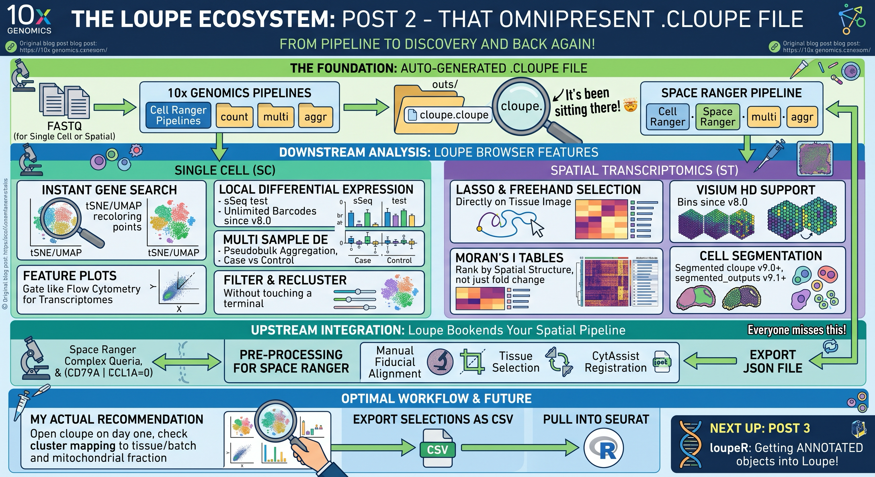
Where the file comes from 📂 Link to heading
.cloupe generation is built into the pipelines rather than bolted on afterwards. Per the Cell Ranger outputs documentation and the Space Ranger outputs overview, you get one from:
-
cellranger count,cellranger multiandcellranger aggr -
spaceranger countandspaceranger aggr
For Visium HD run through Space Ranger v4.0 or later, there is a second one. Space Ranger now runs nucleus and cell segmentation by default on Visium HD and Visium HD 3’ H&E samples, and writes a cloupe.cloupe into the segmented_outputs/ folder containing segmented cells rather than bins. That file requires Loupe Browser v9.0 or later to open, which is a common source of confusion when someone is running an older Loupe install.
There are a few cases where you will not get a file, and knowing them saves a confused half hour. The Space Ranger release notes document the first of these:
-
Visium HD custom bin sizes below 8 µm do not produce a
.cloupe. If you set--custom-bin-sizeto 4 or 6, expect no Loupe file for that binning -
Feature Barcode only runs with fewer than ten antibodies skip secondary analysis entirely, and therefore skip the
.cloupe -
spaceranger aggrdoes not support Visium HD at all
What is actually inside 📦 Link to heading
The container holds the full counts matrix, the precomputed secondary analysis, and for spatial data the imaging layer: graph based clustering, K-means from K=1 to K=10, UMAP and t-SNE, and for Visium a tiled tissue image so that zooming from whole section to individual spot stays instant.
Note that Cell Ranger v9.0 changed the default for cellranger aggr to output UMAP instead of t-SNE, since UMAP benchmarked roughly two and a half times faster. If you want t-SNE back you pass --enable-tsne. For cellranger multi, t-SNE is still calculated and available in the .cloupe regardless. The Cell Ranger release notes track these changes.
The analysis capabilities 🧮 Link to heading
This is where the “just a viewer” characterisation falls apart. Loupe computes. The single cell navigation tutorial walks through most of what follows using a public lung cancer dataset.
Feature expression and scaling. Search any gene, and the projection recolours immediately. You can switch between Linear, Log2 and LogNorm scaling, and the LogNorm implementation deliberately matches Seurat and Scanpy: ln(10000 * (feature count / barcode count) + 1). This matters because it means a violin plot you eyeball in Loupe is comparable to the one you will generate in R rather than being on some proprietary scale.
For multi-gene feature lists you get Feature Max, Min, Sum and Avg as combination modes, which makes module scoring style questions tractable without leaving the interface.
Differential expression. Runs locally, on your laptop, on the full dataset. Since v8.0 there is no barcode limit, and a progress bar with a time estimate and a cancel button, which was a meaningful quality of life improvement. Three comparison modes are available: selected clusters against the entire dataset, selected clusters against each other, and selected clusters across multiple samples.
The statistics are not a toy: Loupe uses the same method as Cell Ranger, an exact negative binomial test using sSeq, switching to edgeR’s fast asymptotic test at high UMI counts. The algorithm is documented publicly and the implementation is open source.
Multi-sample differential expression. Introduced in v7.0, this aggregates barcodes into per-sample pseudobulk columns within each cluster before running sSeq. That is the statistically correct instinct and a pleasant surprise in a point and click tool.
Feature plots. Plot barcodes by the expression of one or two features on a scatter, with linear or log axes. This is functionally flow cytometry for transcriptomes, and if you came from a flow background it will feel immediately natural. It is the fastest way I know to threshold a population and pull out the double positives.
Co-expression. Added in v8.0. Select two feature lists and visualise where they overlap. Useful for pathway versus cell type questions, or for checking whether two markers you assume are co-expressed genuinely are. Not available for ATAC or Multiome datasets.
Advanced Selection. Boolean filtering, which lives under Advanced Selection in the v7.0 and later interface, lets you construct expressions like (CD79A OR CD79B) AND TCL1A = 0 directly. Anyone who has written the equivalent subset() call with WhichCells() and a nested expression will appreciate the difference.
Filtering and reclustering. Now labelled Reanalyze. Subset by cluster membership, UMI count, distinct feature count, mitochondrial UMI fraction, or an uploaded CSV of barcodes, then regenerate clustering and a projection over the filtered data. Since v8.0 this is unlimited in barcode count. One caveat worth flagging: the random seed for graph based clustering changed in v9.0, so reanalysing the same dataset in v9 will give slightly different results than v8 did.
Categories, import and export. Rename and recolour clusters. Import your own annotations from a CSV where the first column holds barcodes and each subsequent column becomes its own category, with the column header becoming the group name. Export DE tables, projection coordinates, and barcode selections. The interoperability documentation covers the exact CSV formats, and the sharing results tutorial covers the export side. This round trip is what makes Loupe part of a real pipeline rather than a dead end.
Import works in the other direction too. Any two dimensional embedding you generate elsewhere, including trajectory layouts, goes in as a three column CSV of barcode, x and y.
The spatial story 🗺️ Link to heading
For spatial work the capability gap between Loupe and a scripted workflow narrows considerably, because so much of spatial exploration is genuinely visual. The spatial navigation tutorial is the entry point.
You get lasso, rectangular and freehand draw selection directly on the tissue image, which is the natural interface for “these spots, the ones inside the tumour margin.” You get the spatial enrichment table ranking features by Moran’s I, so you can sort genes by how spatially structured their expression is rather than by fold change, available for datasets from Space Ranger v1.3 onward. You get spot deconvolution results surfaced for reference free deconvolution from Space Ranger v2.1 and later.
Version by version, the Visium HD support has moved quickly. Loupe v8.0 added visualisation of Visium HD bins alongside the microscopy images. v9.0 added cell segmentation support for Visium HD and Visium HD 3’. v9.1 added support for the 11 mm slides.
Spatial reclustering is supported but only for individual samples processed with spaceranger count. It does not work on samples combined with spaceranger aggr.
Cell annotation arrives in the cloupe 🏷️ Link to heading
This is a recent development worth knowing about. Cell Ranger v9.0 introduced automated cell type annotation as part of cellranger count and cellranger multi, and as a standalone cellranger annotate command. If you pass your existing .cloupe as an input, the pipeline writes out a new annotated .cloupe with the cell types available under Custom Groups. Omit it and the pipeline still runs, but no annotated Loupe file comes out.
Space Ranger v4.1 brought the equivalent to spatial with spaceranger annotate, requiring a Visium HD or Visium HD 3’ library with segmentation enabled.
The original implementation compares each barcode’s expression profile against the CZ CELLxGENE census via 10x Cloud Analysis, which means your data leaves your environment. Cell Ranger v10.1 added the Pan-Human Azimuth model, which runs locally and requires no cloud access. That is a significant change for anyone working with patient derived material under restrictive data agreements.
Treat any of these annotations as a starting point, in exactly the way you would treat SingleR or CellTypist output.
Loupe runs upstream too 🔧 Link to heading
For spatial, Loupe is not only a viewer. The manual fiducial alignment wizard, tissue selection, and CytAssist to microscope image registration all happen in Loupe Browser. You work through the wizard and export a JSON that Space Ranger consumes through --loupe-alignment. Visium HD has its own alignment workflow with automated slide ID detection and fiducial refinement.
When automatic fiducial detection fails, which happens with obscured corners, unusual staining, or difficult tissue morphology, this is the recovery path. Loupe supports three corner alignment when one fiducial is obstructed, auto-levelling for brightness and contrast, and loading a separate overexposed image purely for fiducial detection.
So Loupe sits at both ends of the spatial pipeline, and the upstream half is not optional.
The day one triage workflow ⏱️ Link to heading
Here is how I would actually use this, and it takes twenty minutes.
Before writing any analysis code, open the .cloupe. Colour by the pipeline’s graph based clustering and ask whether the structure looks like biology or like batch. For spatial, ask whether clusters map onto recognisable tissue architecture, because if they do not, something upstream is wrong. Colour by total UMI count and by mitochondrial fraction and see whether any cluster is defined primarily by quality rather than expression. Search three or four markers you are confident about and check they land where they should.
Then lasso anything that looks strange and run differential expression on it. You will learn more about the dataset in those twenty minutes than in the first two hours of scripted QC, because you are looking at the data rather than at summary statistics computed from it.
Finally, export any selection you care about as a barcode CSV, read it into R, and subset your Seurat object on it. The exploration was fast and disposable. The analysis that follows is scripted and permanent. That division is the entire point.
Documentation 📚 Link to heading
What’s next Link to heading
Post 3 covers loupeR, the R package that turns a Seurat object into a .cloupe. That is the direction that matters most in practice: your integrated, annotated, subclustered analysis reaching the people who will never open R.