The .cloupe file that Cell Ranger writes into outs/ is raw pipeline output. Default graph based clustering, no integration, no batch correction, no annotation, no subclustering. It represents the state of your dataset roughly forty minutes after sequencing finished.
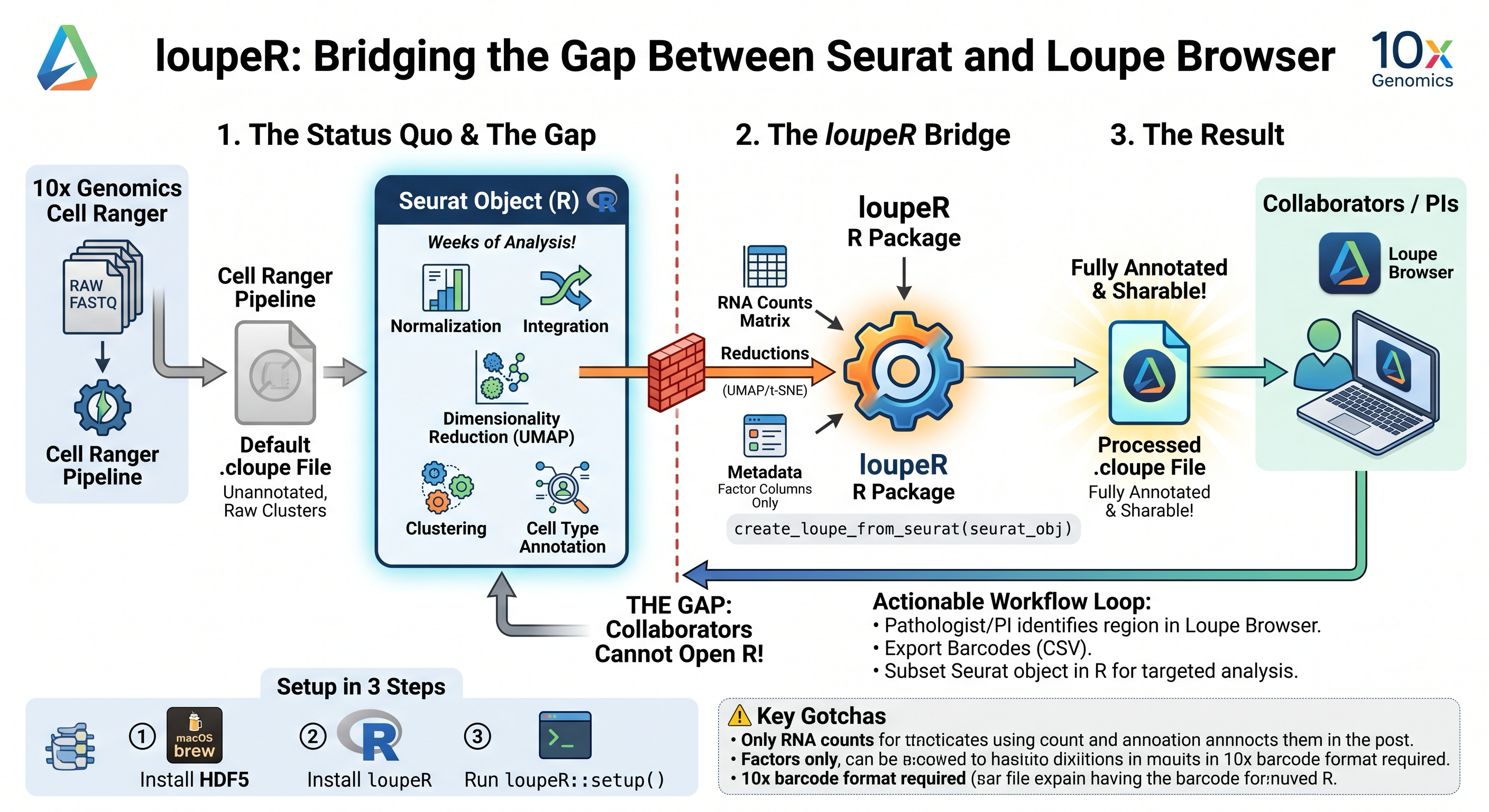
Your actual analysis lives somewhere else entirely. It lives in a Seurat object that has been through QC filtering, normalisation, integration across ten samples, careful manual annotation informed by three literature searches, and a subclustering pass that took a week to get right.
None of that reaches Loupe Browser by default. Which means none of it reaches the collaborators who can only open Loupe.
loupeR closes that gap. It is an R package built and maintained by 10x Genomics that converts Seurat objects into .cloupe files, and it is genuinely straightforward once you know the half dozen things that will otherwise cost you an afternoon. The official tutorial is the reference for everything below.
Installation 🛠️ Link to heading
loupeR needs HDF5 on your system, plus the hdf5r R package and Seurat.
# System dependency
# macOS:    brew install hdf5
# Windows:  .\vcpkg install hdf5

install.packages("hdf5r")
install.packages("Seurat")
install.packages("remotes")
There are two installation routes. The first downloads a platform specific tarball from the releases page with the louper executable pre-bundled, then installs it from source. The second installs from GitHub and fetches the executable separately:
remotes::install_github("10XGenomics/loupeR")
loupeR::setup()
setup() downloads the louper binary and prompts you to accept the 10x end user licence agreement. You type y and press enter. Until you do, loading the package will simply tell you to call setup().
The binary lands in your tools::R_user_dir directory by default. If you need it somewhere specific, for a shared cluster environment or a containerised pipeline, set the LOUPER_USER_DATA_DIR environment variable.
One note for anyone automating this: interactive licence acceptance is a genuine obstacle to putting loupeR inside a Nextflow or Snakemake pipeline. 10x explicitly invites you to contact their support if that is blocking you, which suggests there is a documented workaround they will share on request.
The simple path ⚡ Link to heading
For a standard Seurat object, conversion is one call.
library(loupeR)

seurat_obj <- readRDS("data/integrated_annotated.rds")

create_loupe_from_seurat(
  seurat_obj,
  output_dir  = "outputs",
  output_name = "integrated_annotated"
)
You get integrated_annotated.cloupe. Full argument list:
create_loupe_from_seurat(
  obj,
  output_dir      = NULL,
  output_name     = NULL,
  dedup_clusters  = FALSE,
  feature_ids     = NULL,
  executable_path = NULL,
  force           = FALSE
)
Two arguments deserve attention. dedup_clusters = TRUE collapses clusterings that are numerically identical, which is genuinely useful given that a typical Seurat object carries seurat_clusters alongside RNA_snn_res.0.5 containing exactly the same assignments. Without it, your collaborator opens the file and sees four categories that are all the same thing.
feature_ids accepts a character vector of Ensembl IDs, and passing it makes gene identity unambiguous in the resulting file. There is a helper for pulling them out of standard 10x output:
feature_ids <- read_feature_ids_from_tsv(
  "path/to/filtered_feature_bc_matrix/features.tsv.gz"
)

create_loupe_from_seurat(seurat_obj, feature_ids = feature_ids)
The general path 🧱 Link to heading
create_loupe_from_seurat() is a convenience wrapper. The function underneath is create_loupe(), and it takes raw components rather than a Seurat object:
create_loupe(
  count_mat,
  clusters           = list(),
  projections        = list(),
  output_dir         = NULL,
  output_name        = NULL,
  feature_ids        = NULL,
  executable_path    = NULL,
  force              = FALSE,
  seurat_obj_version = NULL
)
It wants a sparse dgCMatrix of counts, a list of factors holding per-barcode assignments, and a list of matrices with dimensions barcodes by 2.
This is the interesting function, because it is object agnostic. There are helpers to extract the pieces from a Seurat object if that is where you are starting:
clusters    <- select_clusters(seurat_obj)
projections <- select_projections(seurat_obj)

create_loupe(
  count_mat   = counts,
  clusters    = clusters,
  projections = projections,
  output_name = "custom_build"
)
But nothing forces the input to come from Seurat. If you can produce a sparse counts matrix, a list of factors, and a two dimensional embedding, you can build a .cloupe. That covers SingleCellExperiment objects, anything you have exported from AnnData, or an entirely bespoke pipeline.
This is where the “any transcriptomics data” claim gets interesting, and also where it needs qualifying, which brings us to the constraints.
What actually gets carried over 📋 Link to heading
This is the part that surprises people, so it is worth being precise.
Counts only, RNA assay only. create_loupe_from_seurat() passes the active counts matrix. As the documentation states plainly, SCTransform residuals, integrated assays, and any normalised data layer are not stored. Loupe recomputes its own normalisation from the counts. So if your integration lives in an integrated assay, the expression values your collaborator sees are the uncorrected ones. Your clustering and your UMAP still reflect the integration, because those came across, but the expression layer does not.
Factor columns only. Only factors in meta.data become Loupe categories. A character column of cell type annotations, which is what most people produce, is silently ignored. Convert before you convert:
seurat_obj$cell_type <- as.factor(seurat_obj$cell_type)
seurat_obj$sample_id <- as.factor(seurat_obj$sample_id)
seurat_obj$condition <- as.factor(seurat_obj$condition)
Two dimensional projections only. Each entry in projections must be barcodes by 2. A 30 dimensional PCA will not go across as-is; take the first two columns or leave it out.
The gotchas, ranked by how often they bite ⚠️ Link to heading
Barcode formatting is the number one issue on the repository, by a wide margin. loupeR validates that your barcodes are 10x format: sixteen characters from ACGT, followed by an optional GEM well suffix, with optional additional prefix or suffix. What breaks is the standard result of merging samples in Seurat, where barcodes come out looking like Sample01_AAACCCACAACGCACAG-1. That prefix pattern, which Seurat produces by default, trips the validator with an unhelpful message about barcodes needing to begin with base pairs.
The fix is to reformat before conversion, and the safe move is to move sample identity out of the barcode string and into a metadata factor where it belongs anyway.
Cluster grouping cap. No cluster can have more than 32,768 groupings. In practice this bites when a metadata column that is not really a clustering, like a per-cell barcode identifier or a continuous variable that got coerced to factor, ends up in the selection. Check what select_clusters() picked up before you convert.
Version pairing. loupeR releases track Loupe Browser releases, and the repository maintains a compatibility table. Files from loupeR require Loupe Browser v7.0 or later at minimum. If a collaborator cannot open your file, mismatched versions is the first thing to check. The Loupe Browser release notes also log loupeR updates alongside the browser ones, which is a convenient single place to watch.
Visium and Xenium. These are enabled but explicitly not fully supported. Their barcodes are formatted differently, and while loupeR v1.1.2 added scripts to handle them, only expression data comes across. The images do not. For spatial data where the tissue image is the entire point, the pipeline generated .cloupe from Space Ranger remains the better path.
The honest reality check 🎯 Link to heading
It is tempting to describe loupeR as unlocking Loupe Browser for all transcriptomics data, and the architecture of create_loupe() almost supports that reading. But the barcode validator is the real gate, not the object class, and 10x’s own documentation states the prerequisite plainly: a 10x Gene Expression dataset, 3’, 5’ or Flex.
You can get non-10x data through. It means constructing barcode strings that satisfy the validator, which is data wrangling that 10x explicitly does not support. For a Smart-seq dataset or a public matrix with arbitrary cell identifiers, you are essentially manufacturing fake 10x barcodes and keeping a mapping table. That works, and it is not something to build a lab workflow on.
Be accurate with collaborators about which path you are on.
The round trip 🔄 Link to heading
The workflow that makes this genuinely valuable rather than merely convenient runs in both directions.
You convert your annotated object and send the .cloupe. Your collaborator, who knows the tissue, opens it and lassos a region that looks wrong to them, or a population they recognise that your clustering split in two. They export that selection as a barcode CSV, in the format described in the interoperability documentation, and send it back.
selection <- read.csv("collaborator_selection.csv")

# First column holds barcodes by Loupe convention
region_cells <- selection[[1]]

seurat_obj$expert_region <- ifelse(
  colnames(seurat_obj) %in% region_cells,
  "selected",
  "other"
)

Idents(seurat_obj) <- "expert_region"
markers <- FindMarkers(seurat_obj, ident.1 = "selected")
That is domain expertise flowing directly into a computational pipeline, in a form you can immediately test statistically. It is a far better use of a collaborator’s knowledge than asking them to describe the region in an email and then guessing.
Where this leaves the series 🧩 Link to heading
Three posts, one file format. Loupe Browser as the reconnaissance layer with a very short loop between question and answer. .cloupe files already sitting in every pipeline output directory, waiting. And loupeR as the bridge that carries your real analysis across to the people who need to see it but cannot open your R session.
None of it replaces scripted, reproducible analysis. All of it removes friction from the parts of the work that were never going to be scripted anyway.