Open a .ipynb File in a Text Editor Link to heading
Go ahead. I’ll wait.
What you’ll see is raw JSON. Cell metadata objects. Kernel specification blocks. And if you’ve run any plots, you’ll find base64-encoded PNG images embedded directly in the file: thousands of characters of gibberish that represent your UMAP.
Now open an RMarkdown file in a text editor. It’s just text. YAML header at the top, prose in between, code in fenced blocks. Human-readable, diffable, greppable.
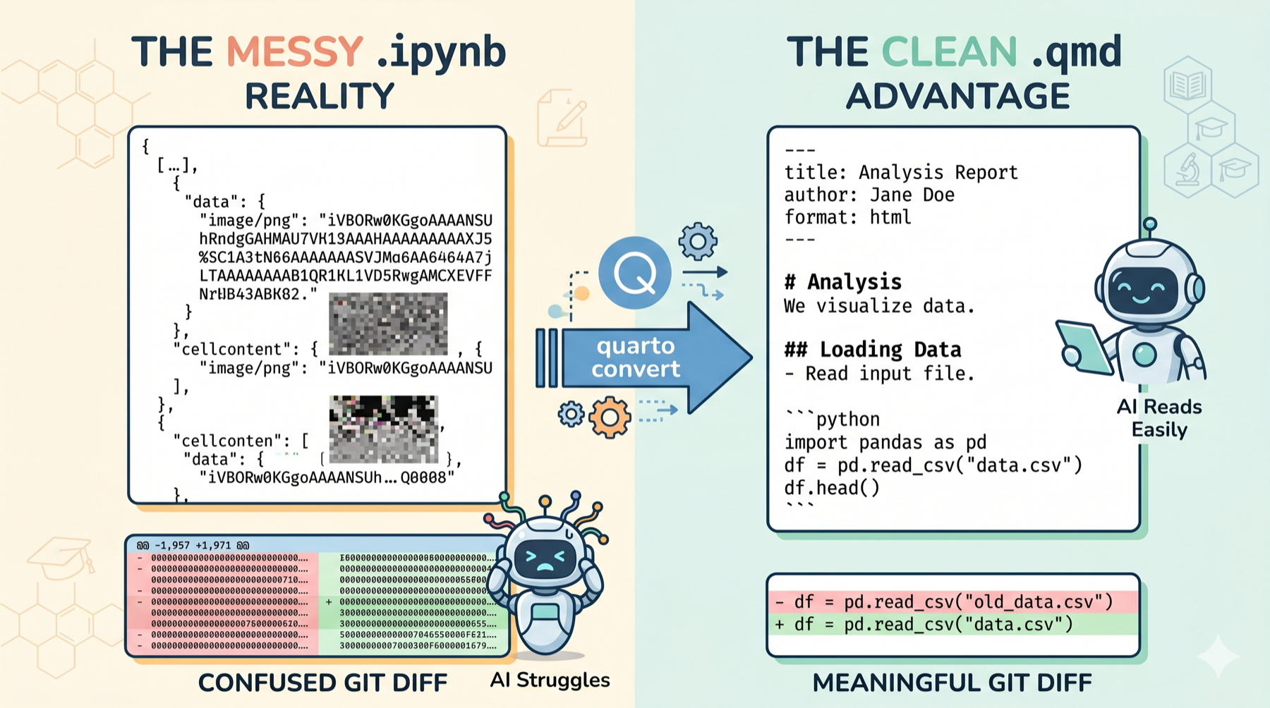
If you’ve spent any time with RMarkdown or Quarto in R, you already know that notebooks don’t have to be like this. And with Quarto’s native Python support, they no longer have to be.
What’s Actually Wrong with .ipynb Link to heading
Jupyter notebooks are excellent for one thing: interactive exploration. You write a line of code, run it, see the output immediately, iterate. For early-stage data exploration, there’s nothing better.
But .ipynb has fundamental design problems that become serious the moment you move beyond exploration:
Version control is a nightmare. Because .ipynb files are JSON with embedded outputs, every time you re-run a cell, the output changes, even if the code didn’t. Your git diff shows thousands of lines of changed base64 image data, making code review essentially impossible. You can strip outputs before committing, but that requires discipline and tooling that most researchers don’t set up.
Reproducibility is fragile. Jupyter lets you run cells in any order. Cell 5 might depend on a variable defined in Cell 3, but you ran Cell 7 in between and overwrote it. The notebook shows green checkmarks everywhere, but if you restart the kernel and run top-to-bottom, it breaks. This out-of-order execution problem has bitten every Jupyter user at least once.
Collaboration is painful. Try merging two branches that both modified the same notebook. The JSON structure means merge conflicts are cryptic and nearly impossible to resolve manually. Most teams resort to “only one person edits the notebook at a time,” which defeats the purpose of version control.
The format is hostile to LLMs. This is the angle that surprisingly few people talk about, but it matters increasingly in 2026. When you ask Claude or Copilot to help with a Jupyter notebook, the LLM has to parse JSON metadata, cell type identifiers, execution counts, and embedded outputs just to find your actual code. With a .qmd file, the LLM sees exactly what you see: markdown and code blocks. The quality of AI-assisted coding improves dramatically when your source format is plain text.
What Quarto Brings to Python Link to heading
Quarto is the successor to RMarkdown, built by Posit (formerly RStudio) with first-class support for Python, R, Julia, and Observable. The key insight is simple: your analysis document should be plain text.
A .qmd file looks like this:
---
title: "scRNA-seq Quality Control"
author: "Badran Elshenawy"
format: html
jupyter: python3
---

## Loading the Data

```{python}
import scanpy as sc
adata = sc.read_h5ad("pbmc3k.h5ad")
print(f"Loaded {adata.n_obs} cells, {adata.n_vars} genes")
```

## Filtering Low-Quality Cells

We remove cells with fewer than 200 genes detected.

```{python}
#| label: fig-qc
#| fig-cap: "QC violin plots before filtering"
sc.pl.violin(adata, ['n_genes_by_counts', 'total_counts', 'pct_counts_mt'])
```
That’s it. Plain markdown with Python code blocks. YAML header for metadata. Special comments (#|) for cell-level options like figure labels and captions. Everything is human-readable, and everything diffs cleanly in git.
The Features You’ve Been Missing Link to heading
If you’re coming from RMarkdown, you’ll feel right at home. Quarto brings all the features that make RMarkdown powerful to your Python workflow:
-
Cross-references:
@fig-qcautomatically links to your labelled figure, with numbering handled for you -
Citations: integrate with .bib files for proper academic referencing
-
Multi-format rendering: one source file produces HTML, PDF, Word, or reveal.js slides with a single command change
-
Table of contents, code folding, tabsets: all the interactive HTML features that make reports navigable
-
Parameterised reports: change a variable in the YAML header, re-render the entire analysis with different inputs
None of these exist natively in Jupyter notebooks. You can hack some of them together with extensions, but it’s never seamless.
The Practical Workflow Link to heading
There are two ways to use Quarto with Python, and both are valid:
Approach 1: Write in .qmd from the start. If you’re using VS Code with the Quarto extension, you get code completion, cell-at-a-time execution, and live preview side-by-side. The experience is similar to working in RStudio with RMarkdown: write, run, see output, iterate.
# Live preview while you work
quarto preview analysis.qmd

# Render to final format
quarto render analysis.qmd --to html
Approach 2: Explore in Jupyter, convert for production. Use Jupyter for your messy exploration phase: try things, plot things, iterate fast. When you’re ready to create a reproducible document, convert:
quarto convert exploration.ipynb # produces exploration.qmd
Then clean up the .qmd, add cross-references and narrative, and render your final report. You get the best of both worlds: Jupyter’s interactivity for exploration, Quarto’s rigour for production.
The LLM Argument Link to heading
I want to spend a moment on this because it’s genuinely underappreciated.
In 2026, most of us are using LLMs to help write and debug code. The quality of that help depends heavily on how well the LLM can understand your source files. A .qmd file is the most LLM-friendly format you can write your analysis in: it’s plain text, the code is clearly delineated, and the narrative context helps the LLM understand what you’re trying to do.
I’ve been using Claude Code with custom Skills for over a year now, and the difference between asking it to work with a .qmd file versus a .ipynb file is night and day. With .qmd, Claude can read the whole document, understand the analysis flow, suggest improvements, catch errors, and write new sections that integrate seamlessly. With .ipynb, it’s fighting the format just to find the code.
If you’re investing in LLM-assisted workflows, and in bioinformatics in 2026, you should be, .qmd is the format that maximises that investment.
The Bottom Line Link to heading
Jupyter notebooks aren’t going away, and they shouldn’t. They’re still the best tool for interactive exploration and rapid prototyping. But for reproducible analysis documents, collaborative projects, and anything that touches version control, .qmd is the superior format.
For R users migrating to Python, this is the easiest win in the entire series. You already understand the philosophy. You already know why plain text notebooks are better. Quarto just lets you bring that philosophy with you into the Python world, with zero compromises.
This wraps up the foundations of the series: polars for data wrangling, uv for environments, and Quarto for notebooks. With these three tools, the ergonomic gap between R and Python essentially disappears.
Now the real fun begins. Next up, we dive into the scverse ecosystem itself: scanpy, CellTypist, scVelo, and real analysis pipelines. Biology first, code second, same as always.
See you there.